
1. Introduction
This document is an accompaniment to the following inertial measurement units (IMUs) from Shimmer:
The Shimmer3 Wireless Sensor Unit contains accelerometers, a gyroscope and a magnetometer to enable a complete 9 DoF solution. There are two accelerometers, providing the option for wide range or low noise measurements, allowing the user to tailor the configuration to the needs of the application.
The Shimmer3R Wireless Sensor Unit, the current generation of Shimmer3, offers the same functions with newer sensors: low-noise and wide-range accelerometers, a gyroscope, a magnetometer and a pressure sensor, plus a ±200 g high-g accelerometer on the IMU. The sensors are described in Shimmer3R Capabilities. The theory and applications in Sections 3 to 5 apply to both.
It is intended that users refer to this document to help getting started with measuring and processing kinematic data using the Shimmer platform. The document contains theoretical and practical information regarding kinematic signals and sensors, along with a brief description of some common applications for these signals. It also includes signal quality specifications. Please refer to the Table of Contents on the previous page to find the parts of this document that are most relevant to your needs.
2. General Information
2.1. Pre-Requisites
- A Shimmer3R or Shimmer 3 device programmed with appropriate firmware. A Shimmer3R ships with LogAndStream for Shimmer3R, which logs and streams. For example for Shimmer 3, LogAndStream (v0.6.0 or greater) can be used to log data or stream data over Bluetooth while SD Log (v0.12.0 or greater) can be used to log data to the SD card; both are available for download from www.shimmersensing.com.
3. Inertial Measurement Units
This sections provides a brief introduction to IMUs (sometimes known as kinematic sensors) and the signals that they measure.
3.1. Accelerometer
The acceleration, a, of a body can be defined as its rate of change of velocity and it is directly proportional to the forces, F, acting on the body:
.
An accelerometer is a device which measures acceleration due to all forces acting on the device. Forces acting on a device include both the gravitational force due to the mass of the earth as well as any inertial forces which may be applied to the device.
The two primary components of acceleration are, thus, inertial and gravitational acceleration. Thus, the total acceleration, , measured by the device is the vector sum of these components:
,
where is the inertial component and is the gravitational component.
Inertial acceleration
Inertial acceleration occurs due to the application of a force other than gravity to a body. Unless a body is completely motionless or moving with a constant velocity, there are inertial forces acting on it. These forces give rise to inertial acceleration. This acceleration is defined as the rate of change of velocity of the body in motion. It is measured in units of m/s2.
Acceleration due to gravity
Gravity is a natural phenomenon by which physical bodies attract each other with a force proportional to their masses. Gravity is most familiar as the agent that gives weight to objects with mass and causes them to fall to the ground when dropped.
The units of gravity are m/s2. Thus, it is a form of acceleration and is measured by an accelerometer. When an accelerometer is completely stationary (i.e. there is no inertial acceleration acting on the device), it measures a constant acceleration equal in magnitude to the acceleration due to gravity (9.81 m/s2 approx). This is often referred to in units labelled “g”, where 1 g ≈ 9.81 m/s2.
It is a common misconception to assume that the direction of the gravity vector measured by an accelerometer is vertically downwards; this is incorrect. In fact, the measured vector of acceleration due to gravity points vertically upwards from the Earth’s surface.
A simple example to help you remember that this is the case is the observation that an accelerometer in free-fall records an acceleration of zero. In this case, the downward inertial acceleration due to motion equals the upward gravitational acceleration.
A good way to understand why the measured acceleration due to gravity points in an upward direction is to imagine that an accelerometer is a hollow cube with a ball inside, as illustrated in Figure 3‑1. The six faces of the cube will measure acceleration in the positive and negative directions of the three sensing axes as illustrated by the X, Y and Z directions in the figure. To begin with, imagine that the ball is weightless – it is suspended in the middle of the hollow cube and not affected by gravity.
In Figure 3‑1, the accelerometer has no forces acting on it – i.e. no inertial acceleration due to movement and no gravitational acceleration. The acceleration measured in each of the axes, , and , will be zero. This is the case when the device is in free-fall.
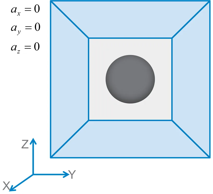
Figure 3‑1 Accelerometer in free-fall
Now, continuing to ignore gravity by assuming that the ball is weightless, imagine that the cube is moved to the right; i.e. acceleration in the positive Y-direction, as shown in Figure 3‑2. The accelerometer will detect acceleration in the positive Y-direction by feeling the suspended ball press against the opposite face of the box.
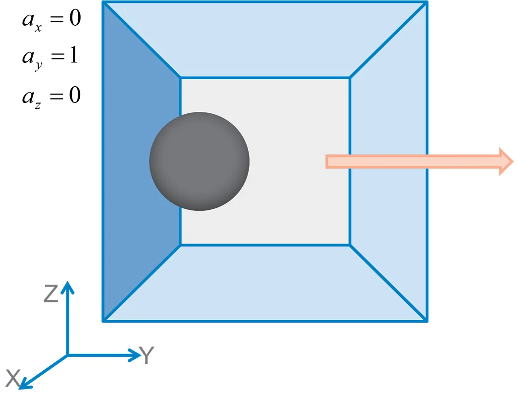
Figure 3‑2 Acceleration in positive Y-direction
Now, let’s lift the assumption that the ball is weightless and include the effect of gravity. If the accelerometer is motionless, the ball will rest on the bottom face of the hollow cube. Just as you have seen that positive acceleration in the Y-axis was detected by the ball pressing against the opposite face, in this case, positive acceleration due to gravity in the Z-axis will be detected by the ball pressing against its opposite face. Thus, it is clear that acceleration due to gravity, measured by the accelerometer, points in an upward direction.
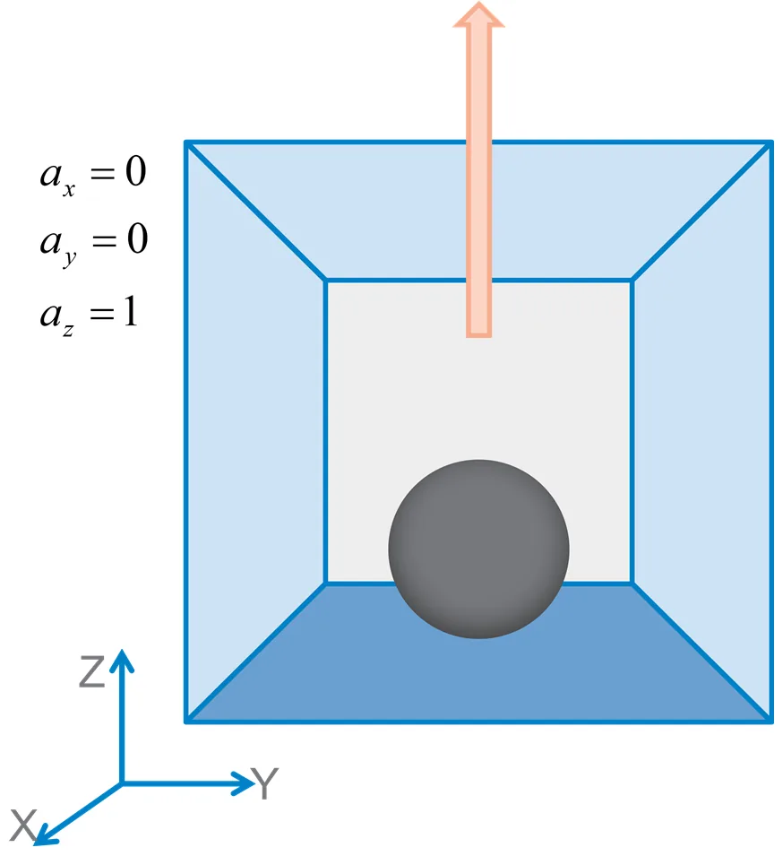
Figure 3‑3 Accelerometer measuring gravity in upward positive Z-direction
Measuring 3D Acceleration
The Shimmer3 is equipped with tri-axial accelerometers. The default representation of its reference axes, as assumed in Shimmer applications, is arranged as shown in Figure 3‑4. Thus, the acceleration measured by the Shimmer device has three components, one in each of the X-, Y- and Z-axes.
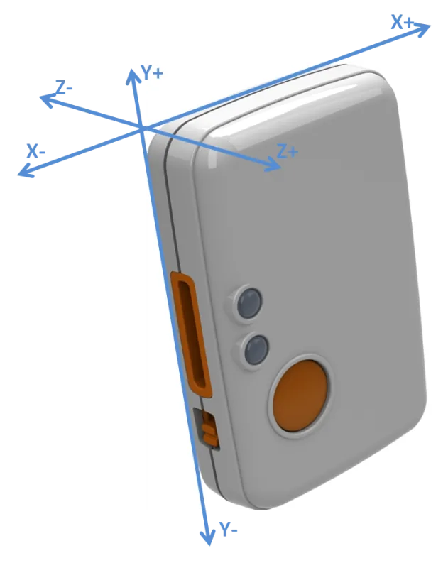
Figure 3‑4 Shimmer3 default axis directions
To understand how the acceleration is distributed across the axes, we consider, first, a single axis (uni-axial) accelerometer.
Uni-axial accelerometer
A uni-axial accelerometer measures the sum of the inertial acceleration component and gravitational acceleration component acting along its single measuring axis. The left side of Figure 3‑5 shows a uni-axial accelerometer, with measurement axis, , attached to a leg segment. There is an inertial acceleration of acting on the segment, as illustrated. The gravitational acceleration vector, , is also included in the figure.
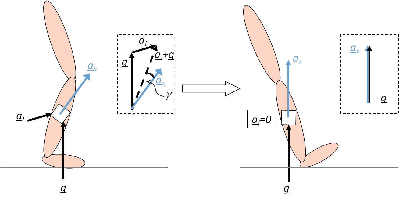
Figure 3‑5: Uni-axial accelerometer attached to a leg segment
In the insert at the left side of the figure, the sum of the inertial and gravitational acceleration vectors is illustrated by a dashed arrow, . This vector is the total acceleration acting on the device. The sensor axis, , measures a component of this acceleration, whose magnitude is given by:
,
where denotes the magnitude of the vector , and is the angle between the measurement axis, , and the total acceleration vector*,* . Alternatively, can be written as:
,
where and are the angles that the axis, , makes with the inertial acceleration vector, , and the gravity vector, , respectively, is the magnitude of inertial acceleration vector and m/s2 is the magnitude of the gravity vector.
In the right side of Figure 3‑5, the leg segment (and, hence, the uni-axial accelerometer) has moved and come to rest in the position shown. In this case, the inertial acceleration is zero (). Thus, gravity is the only acceleration component felt by the device. Due to the rotation of the sensor cause by the movement of the leg segment, the accelerometer measurement axis is now perfectly aligned with the gravity vector. In this case, , as illustrated in the insert on the right side of the figure.
Bi-axial accelerometer
A bi-axial accelerometer consists of two uni-axial accelerometers arranged at a right angle to one another, as illustrated in Figure 3‑6. This device measures the sum of the inertial acceleration component and gravitational acceleration component acting along each of its two measuring axis. The bi-axial accelerometer in Figure 3‑6 is measuring acceleration under the same conditions as described for Figure 3‑5.
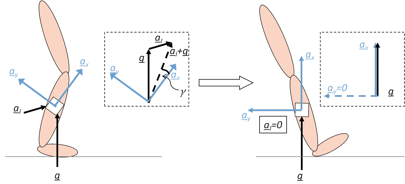
Figure 3‑6: Bi-axial accelerometer attached to a leg segment
The insert at the left side of the figure shows the vector sum of the inertial and gravitational acceleration components, as in Figure 3‑5. This time, the acceleration will be measured in two axes. However, the acceleration measured by the X-axis () will be exactly the same as that measured by the uni-axial accelerometer in the same position; the two axes of the accelerometer act independently of each other. The Y-axis () will measure the acceleration perpendicular to , whose magnitude is given by:
,
where is the angle between the measurement axis, , and the total acceleration vector*,* , as described previously (note, that this angle is defined from the X-axis). Alternatively, can be written as:
,
where and are the angles that the axis, , makes with the inertial acceleration vector, , and the gravity vector, , respectively.
Now, consider the right side of Figure 3‑6, in which the inertial acceleration is zero and the X-axis is parallel to the gravity vector. In this situation, the Y-axis is perpendicular to the gravity vector (i.e. at an angle of 90°) and, thus, the Y-axis will measure because the gravity vector has no component perpendicular to itself. Indeed, the component of any vector acting perpendicular to the vector itself is always zero.
The total acceleration measured by the bi-axial accelerometer may be written as a vector:
.
A bi-axial accelerometer can be used to measure the inclination angle of the body to which it is attached, if its measurement axes are located in the plane of the gravity vector and the only force acting on the device is gravity. In the case shown on the right-hand side of Figure 3‑6, and the angle of inclination, , of the device, with respect to the gravity vector is given by:
.
Tri-axial accelerometer
A tri-axial accelerometer is formed of three mutually orthogonal uni-axial accelerometers (i.e. three accelerometer components arranged such that each axis is at a right angle to the other two axes). As in the case of the uni-axial and bi-axial accelerometers, each axis measures a certain proportion of both the gravitational acceleration and the inertial acceleration. The proportions measured by a given axis depend on the angles between that axis and the directions of the acceleration components. The total acceleration vector can be written as:
,
where the same notation that has previously been used for the X- and Y-axes is followed for the Z-axis.
3.2. Angular rate gyroscope
The angular velocity of a body can be described as the rate at which the object is rotating, in terms of both the speed of rotation and the axis about which it is rotating. A rate gyroscope can be used to measure angular velocity.
The Shimmer3 is equipped with a tri-axial rate gyroscope to measure angular velocity in three dimensions. To understand what component of angular velocity each of the three axes measures, it is useful to, first, consider a uni-axial gyroscope.
Uni-axial rate gyroscope
A uni-axial rate gyroscope measures the angular velocity acting along a single measuring axis. Figure 3‑7 shows a uni-axial gyroscope attached to a rotating plate, rotating with angular velocity , whose magnitude is and direction is perpendicular to the plate, as illustrated.
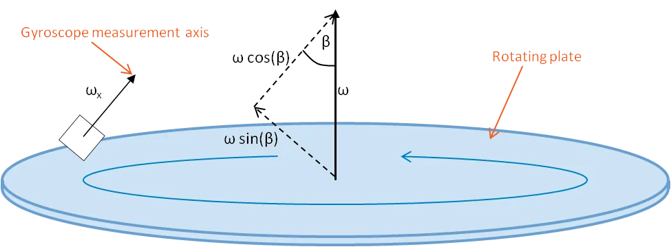
Figure 3‑7: Uni-axial rate gyroscope attached to a rotating plate
The angular velocity measured by the gyroscope, whose measurement axis, , makes an angle, , with the axis about which the plate is rotating, is given by:
,
where
is the magnitude of the angular velocity vector component along the measuring axis of the rate gyroscope,
is the inclination of the measuring axis with respect to the angular velocity vector,
is the magnitude of the angular velocity acting on the sensor.
If the measurement axis is aligned parallel with the rotation axis, then the measured angular velocity will be equal to . If, on the other hand, the measurement axis is perpendicular to the rotation axis, then it will measure an angular velocity of zero.
Tri-axial rate gyroscope
A tri-axial rate gyroscope is formed by three orthogonal uni-axial rate gyroscopes. A 3-dimensional angular velocity vector is obtained from a tri-axial rate gyroscope. The angular velocity vector measured by a tri-axial rate gyroscope is given by:
,
where , and are the angles that the measurement axes, , and make with the rotation axis, respectively.
3.3. Magnetometer
Magnetic fields describe the influence of electric currents and magnetic materials on objects around them. The Earth has its own permanent magnetic field whose direction runs from the magnetic South pole to the magnetic North pole and which influences all magnetic objects. This magnetic field can be exploited to determine the heading of an object, using a compass. Large metal objects and sources of electromagnetic interference (such as lights or electronic devices) can distort the local effect of the Earth’s magnetic field, resulting in heading errors, so it is best to use compasses as far away from these sources of interference as possible.
A magnetometer is a sensor which is used to measure the direction and/or the strength of the local magnetic field. If the only magnetic field acting on the magnetometer is the Earth’s magnetic field, then it can be used as a compass to determine the direction in which the sensor is facing, relative to the Earth’s magnetic North pole.
The Earth’s magnetic field does not act parallel to the Earth’s surface. Instead, there is a magnetic inclination (also known as magnetic dip) angle, which causes the compass needle to point upwards or downwards (relative to the horizontal plane of the Earth’s surface), depending on where in the world the compass is. At the magnetic equator, the angle is zero and the magnetic field does act exactly parallel to the Earth’s surface. In the Northern hemisphere, the North end of the compass needle begins to point downwards more and more as one approaches the magnetic North Pole. In the Southern hemisphere, the North end of the compass needle points increasingly upwards as one approaches the magnetic South pole. When using a magnetometer to measure the magnetic field in three dimensions, the appropriate magnetic inclination angle for the geographic location should be taken into account. For example, in Dublin, Ireland, the angle is approximately 68°.
The Shimmer3 is equipped with a tri-axial magnetometer to measure the local magnetic field in three-dimensions. To understand how the magnetic field measurement is distributed over the three sensing axes, it is useful to, first, consider a uni-axial magnetometer.
Uni-axial magnetometer
A uni-axial magnetometer measures the magnetic field vector acting along its measuring axis. Figure 3‑8 shows a uni-axial magnetometer attached to a leg segment.
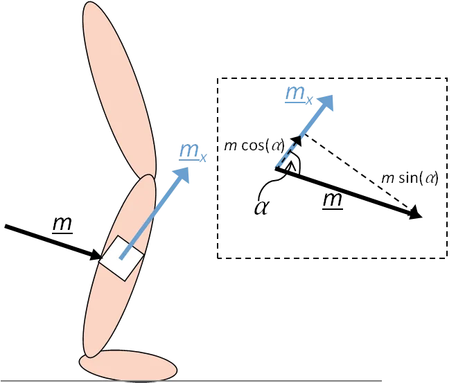
Figure 3‑8: Uni-axial magnetometer attached to a leg segment
The magnetic field measured by the magnetometer, whose measurement axis, , makes an angle, , with the magnetic field vector, , is given by:
,
where
is the magnitude of the magnetic field vector component along the measuring axis of the magnetometer,
is the angle between the magnetometer measuring axis and the magnetic field vector,
is the magnitude of the magnetic field acting on the sensor.
If the measurement axis is aligned parallel with the magnetic field vector, then the measured magnetic field component will be equal to . If, on the other hand, the measurement axis is perpendicular to the magnetic field vector, then it will measure a magnetic field of zero.
Bi-axial magnetometer
A bi-axial magnetometer consists of two uni-axial magnetometer components arranged perpendicular to each other. The magnetic field component measured by the X-axis remains unchanged from the uni-axial case. The component measured by the Y-axis is given by:
,
where is the same angle that was defined previously and illustrated in Figure 3‑8.
A bi-axial magnetometer can be used to measure the inclination angle of the body to which it is attached, if its measurement axes are located in the plane of the magnetic field vector. In this case, the heading angle, , of the device, with respect to the magnetic field vector is given by:
.
If the local magnetic field is equal to the Earth’s magnetic field (i.e. there are no sources of interference), then is the heading angle of the sensor, relative to the Earth’s magnetic North pole.
Tri-axial magnetometer
A tri-axial magnetometer is formed by three orthogonal uni-axial magnetometers. A 3-dimensional magnetic field vector is obtained from a tri-axial magnetometer. The magnetic field vector, , measured by a tri-axial magnetometer is given by:
,
where , and are the angles that the measurement axes, , and make with the magnetic field vector, , respectively.
4. Inertial Sensor Signals
4.1. The IMU Signal
IMUs, like all sensors, are subject to noise and other errors, like offset bias and axis alignment errors. Furthermore, sensor measurements are limited to values in a finite range, whilst most physical phenomena have an infinite range. Also, if the output of the sensor is digital, quantisation introduces noise in the measurements. Thus, the value measured by any sensor is not exactly equal to the value of the phenomenon being measured.
Uni-axial sensor measurement
For a uni-axial sensor, if the value of the sensed phenomenon along the sensor measurement axis is , then the sensor output, , can be described by:
,
where is the sensor scale factor, is the offset bias and is noise. Ignoring noise, which is usually random and cannot be estimated, the scale factor is the value by which the sensor output will increase for an increase of one unit in the sensed phenomenon and the offset bias is the value of the sensor output when the sensed phenomenon is equal to zero; these quantities can both be estimated by calibrating the sensor1.
Tri-axial sensor measurement
Ideally, a tri-axial IMU should consist of three mutually orthogonal uni-axial sensors (i.e. each axis makes a right angle with the other two axes). However, real sensors tend to be subject to misalignment errors due to minor errors in the placement of sensors, meaning that the sensor axes are not precisely orthogonal to each other. Also, the assumed orientation of the sensor may not be aligned with its true orientation when it is placed inside its casing.
The result of this misalignment error is that it is necessary to define a rotation operation which relates the assumed sensitivity axes with the actual sensitivity axes of the sensor. In fact, the user may define any set of assumed sensitivity axes and calculate the required rotation during the calibration process2. The rotation can be easily described by a rotation matrix, .
For a tri-axial sensor, if the value of the sensed phenomenon vector is , then the sensor output, , can be described by:
,
where
is the sensor output,
is the vector value of the sensed phenomenon,
is the diagonal matrix of sensor axis scale factors,
is the rotation matrix which defines the actual sensor axes (, and ) with respect to the assumed sensitivity axes (, and ),
is the offset bias vector, and
is the noise vector.
The average noise affecting the kinematic sensors on the Shimmer3 is summarised in Section 6.1.
4.2. Kinematic Parameters
The complete kinematics of a body in three-dimensional space can be described using the following 15 variables (Winter, 1990):
Linear displacement of body’s centre of mass (, and ),
Linear velocity of the body’s centre of mass (, and ),
Linear acceleration of the body’s centre of mass (, and ),
Angular displacement of the body in two planes (,),
Angular velocity of the body in two planes (),
Angular acceleration of the body in two planes ().
These parameters can be estimated using IMUs with varying levels of difficulty. For example, linear acceleration and angular velocity can be directly estimated from the accelerometer and gyroscope observations, respectively. Angular acceleration can be determined by calculating the derivative of angular velocity, taking care to deal with high frequency noise introduced by the derivative. Angular displacement can be instantaneously estimated using a stationary accelerometer and/or magnetometer, as outlined in Sections 3.1 and 3.3, whilst sensor fusion of at least accelerometer and gyroscope is required to accurately estimate continuous angular displacement for moving bodies. Linear velocity is the integral of linear acceleration, but measures to eliminate errors due to accelerometer offset bias and noise must be taken to ensure accurate estimation. Finally, estimation of linear displacement requires complicated sensor fusion algorithms; this topic is briefly discussed in Section 5.2.
4.3. Coordinate Systems
The coordinate system used to define the variables above must be defined relative to some reference system; if the coordinate system is defined relative to a constant external reference system, then the reference is known as the global system. One of most commonly used global reference systems is the Earth’s {North, East, Down} frame. If, on the other hand, the coordinate system for one body is described relative to the coordinate system of another body (which may itself be variable), then it is known as a relative system.
For example, imagine that two sensors are attached to a person’s arm, with one below the elbow and the other above the elbow, and the person moves his/her arm whilst walking through a building. The relative kinematics describe the linear and angular displacements, velocities and accelerations between the two arm segments, regardless of where in the building the person is, in which direction they are facing, or whether they are moving or still. The global kinematics describe the linear and angular displacement, velocity and acceleration of each sensor, independent of the other sensor, describing where in the building the person is, etc.
The angular displacement of one coordinate system, relative to another system, can be described by a rotation matrix of dimension, 3×3. For more detail on how to construct this matrix, see (Craig, 1989), for example. There are also other formats for describing the angular displacement between to coordinate systems, including angle-axis, Euler angles and quaternions. The preference for one format over another depends largely on the application and its storage and computational requirements and limitations.
5. Applications of IMUs
The following are examples of problems for which IMU-based solutions are often sought. A very brief outline of the suitability of IMUs for these problems is provided, along with some references to help the new user to get started with investigating these topics. Please note that solutions to these applications are not directly supported by Shimmer and the information below is intended as a starting point for the new user, unfamiliar with the relevant literature.
5.1. Gait analysis
Inertial sensors are ideal for measuring the temporal parameters of gait (stride time, step time, stance time). The following paper describes methods by which this can be achieved using a gyroscope (Greene, McGrath, O’Neill, O’Donovan, Burns, & Caulfield, 2010). Determining spatial parameters (e.g. step length and stride length) from inertial sensors is non-trivial due to the problems of drift associated with double integration of the noisy accelerometer signal. Examples of publications which attempt to estimate the spatio-temporal parameters using inertial sensors include (Doheny, Foran, & Greene, 2010), (Bugané, et al., 2012), (Zijlstra, 2004), (Sabatini, Martelloni, Scapellato, & Cavallo, 2005).
5.2. Displacement estimation
Noise and other error sources (e.g. offset bias) in accelerometers mean that it is not possible to accurately estimate displacement by direct double integration of accelerometer observations alone. Indeed, the problem of estimating displacement is not a trivial one and there is vast literature available on the subject. A recently published review of displacement estimation systems (Harle, 2013) and the references therein provide a good starting point for understanding the subject.
Most successful displacement estimation systems rely on fusion of multiple sensors – including accelerometers, gyroscopes and magnetometers, as well as video, GPS, and infra-red position sensors, to name just a few examples. They also involve elaborate processing of the inertial observations, with Kalman filters and their derivatives being among the most popular approaches, e.g. (Won, Melek, & Golnaraghi, 2010). Other ad hoc approaches, such as the use of zero velocity updates for walking data (Skog, Nilsson, & Handel, 2010), or constrained sensor placement (Yadav & Bleakley, 2011) can also help to limit the growth of errors. The required level of accuracy and, more significantly, the length of time over which accurate continuous displacement estimation is needed, determines how complicated the solution needs to be.
5.3. Orientation estimation
Estimation of the orientation of an object in three-dimensional space can be calculated using IMUs. Using accelerometers and gyroscopes, the orientation of the object, relative to its initial orientation, can be determined. For a full orientation solution, estimating absolute instead of relative orientation, magnetometers are also required. There are many such algorithms in the literature – an example of both a relative algorithm and an absolute orientation algorithm can be found in (Madgwick, Harrison, & Vaidyanathan, 2011).
5.4. Fall detection
Fall detection is a common application of IMUs in healthcare, with concerns about an ageing population generating significant research interest in recent years. A basic but over-simplistic method for detecting falls using an accelerometer alone, would be to calculate the magnitude of the measured acceleration and compare this to a threshold to detect a large spike due to an impact. A recent review on fall detection (Mubashir, Shao, & Seed, 2013) contains a section on various accelerometer-based methods and a comprehensive list of references. Other articles describing how IMUs can be used for fall detection include (Bourke, et al., 2010), (Bourke, O’Donovan, & OLaighin, 2008), (Nyan, Tay, & Murugasu, 2008) and the references therein.
6. Practical Usage Considerations
6.1. Shimmer3 Capabilities
Shimmer3 has been built with three sets of sensors. Which set a unit has depends on when it was made:
| Function | First generation (from 2013) | Second generation (from 2017) | Third generation (from 2022) |
|---|---|---|---|
| Low noise accelerometer | KXRB5-2042 (Kionix) | KXTC9-2050 (Kionix) | KXTC9-2050 (Kionix) |
| Wide range accelerometer | LSM303DLHC (STMicroelectronics) | LSM303AHTR (STMicroelectronics) | LSM303AHTR, or ICM-20948 (TDK InvenSense) on boards without it |
| Magnetometer | LSM303DLHC | LSM303AHTR | LSM303AHTR, or ICM-20948 on boards without it |
| Gyroscope | MPU-9150 (InvenSense) | MPU-9250 (InvenSense) | ICM-20948 |
| Pressure and temperature | BMP180 (Bosch) | BMP280 (Bosch) | BMP280 |
Table 6‑1 Shimmer3 sensor generations
Consensys and the Shimmer APIs detect the fitted sensors and calibrate each correctly, so the generation matters only when comparing raw data between units, or for the detail in the manufacturers’ datasheets. The board revision reference lists the sensors on every board revision.
The figures in the rest of this section are for the first generation. For the second and third generations, from the manufacturers’ datasheets (accelerometer sensitivities in LSB/(m/s²), the unit of the defaults in Default calibration parameters in the Shimmer3/3R User Manual):
| Sensor | Generation | Range | Sensitivity | Other |
|---|---|---|---|---|
| Low noise accelerometer (KXTC9-2050) | Second and third | ±2 g | 660 mV/g (±20 mV) | Noise density 125 µg/√Hz |
| Wide range accelerometer (LSM303AHTR) | Second and third | ±2 g; ±4 g; ±8 g; ±16 g | 1671 LSB/(m/s²) at ±2 g | 14-bit; RMS noise 0.6 mg at ±2 g |
| Wide range accelerometer (ICM-20948, on boards without the LSM303AHTR) | Third | ±2 g; ±4 g; ±8 g; ±16 g | 1671 LSB/(m/s²) (16384 LSB/g) at ±2 g | 16-bit |
| Magnetometer (LSM303AHTR) | Second and third | ±49.152 Ga | 667 LSB/Ga | 16-bit; RMS noise 3 mGa |
| Magnetometer (ICM-20948, on boards without the LSM303AHTR) | Third | ±4900 µT | 0.15 µT/LSB | 16-bit |
| Gyroscope (MPU-9250) | Second | ±250; ±500; ±1000; ±2000 deg/sec | 131 LSB/(deg/sec) at ±250 deg/sec | 16-bit; RMS noise 0.1 deg/sec |
| Gyroscope (ICM-20948) | Third | ±250; ±500; ±1000; ±2000 deg/sec | 131 LSB/(deg/sec) at ±250 deg/sec | 16-bit |
| Pressure (BMP280) | Second and third | 300 hPa to 1100 hPa | Resolution 0.16 Pa (pressure), 0.01 °C (temperature) | RMS noise 1.3 Pa |
Table 6‑2 Second- and third-generation sensor ranges and sensitivities
Low Noise Accelerometer
The output of the low noise accelerometer device on the Shimmer3 is analog. A KXRB5-2042 device from Kionix is used. The following approximate values apply to this device:
Zero-output: 1.5 V.
Full scale range: ±2.0 g.
Sensitivity: 600 mV/g.
Please refer to the manufacturer’s datasheets for detailed information.
Wide Range Accelerometer
The output of the wide range accelerometer device on the Shimmer3 is digital. An LSM303DLHC device from STMicro is used (this chip also gives magnetic sensing output). The following approximate values apply to this device:
Full scale range: ±2.0 g; ±4.0 g; ±8.0 g; ±16.0 g.
Sensitivity, in the 16-bit data the Shimmer records (LSB/(m/s²)): 1631 (±2.0 g); 815 (±4.0 g); 408 (±8.0 g); 135 (±16.0 g). These are the defaults in Default calibration parameters in the Shimmer3/3R User Manual. The datasheet gives 1000, 500, 250 and 83.3 LSB/g for the 12-bit reading, which the sensor places in the upper bits of its 16-bit output, so the recorded data is 16 times larger.
Output: 16 bit output2.
Please refer to the manufacturer’s datasheets for detailed information.
Gyroscope
The output of the gyroscope device on the Shimmer3 is digital. The gyroscope on the MPU-9150 chip from Invensense is used. The following approximate values apply to these devices:
- Full scale range (deg/sec): ±250; ± 500; ±1000; ±2000.
Sensitivity (LSB/(deg/sec)): 131 (±250); 65.5 (±500); 32.8 (±1000); 16.4 (±2000).
Output: 16 bits.
Please refer to the manufacturer’s datasheets for detailed information.
Magnetometer
The output of the magnetometer device on the Shimmer3 is digital. An LSM303DLHC device from STMicroelectronics is used (this chip also gives wide range accelerometer output). The following approximate values apply to this device:
Full scale range (Ga): ±1.3; ±1.9; ±2.5; ±4.0; ±4.7; ±5.6; ±8.1.
Sensitivity (X,Y/Z) (LSB/Ga): 1100/980 (±1.3); 855/760 (±1.9); 670/600(±2.5); 450/400 (±4.0); 400/355(±4.7); 330/295 (±5.6); 230/205 (±8.1).
Output: 16 bits3.
Please refer to the manufacturer’s datasheets for detailed information.
6.2. Shimmer3R Capabilities
All the kinematic sensors on the Shimmer3R are digital, including the low-noise accelerometer, which on Shimmer3 is analogue. The ranges and sampling rates below are those offered in Consensys and the Shimmer APIs. Please refer to the manufacturers’ datasheets for sensitivities and detailed information; calibration in Consensys accounts for the sensitivity of each range.
| Function | Device | Full scale range | Sampling rate |
|---|---|---|---|
| Low noise accelerometer | LSM6DSV (STMicroelectronics) | ±2.0 g; ±4.0 g; ±8.0 g; ±16.0 g | Shared with the gyroscope |
| Gyroscope | LSM6DSV (STMicroelectronics) | ±125; ±250; ±500; ±1000; ±2000; ±4000 deg/sec | 1.875 Hz to 7680 Hz |
| Wide range accelerometer | LIS2DW12 (STMicroelectronics) | ±2.0 g; ±4.0 g; ±8.0 g; ±16.0 g | 12.5 Hz to 1600 Hz (high-performance mode); 1.6 Hz to 200 Hz (low-power mode) |
| Magnetometer | LIS2MDL (STMicroelectronics) | ±49.152 Ga (one range) | 10, 20, 50 or 100 Hz |
| High-g accelerometer (IMU only) | ADXL371 (Analog Devices) | ±200 g | 320, 640, 1280 or 2560 Hz |
| Pressure and temperature | BMP390, or BMP581 on later boards (Bosch) | 300 hPa to 1250 hPa | 0.0015 Hz to 200 Hz |
Table 6‑3 Shimmer3R kinematic sensors
The low noise accelerometer and the gyroscope are one device, so they share a sampling rate. Whatever the sensors allow, the Shimmer samples at no more than 4096 Hz.
Compared with Shimmer3:
- Magnetometer: there is a single range, ±49.152 Ga, so there is no range to choose. It matches the second-generation Shimmer3 magnetometer (LSM303AHTR); the first-generation LSM303DLHC offers ranges up to ±8.1 Ga.
- Gyroscope: a ±125 deg/sec range for slow movements and a ±4000 deg/sec range for fast ones are added.
- High-g accelerometer: this is new, for impacts well beyond ±16 g.
- Data order: Shimmer3R sends pressure before temperature, and its temperature value is 3 bytes rather than 2. Consensys and the Shimmer APIs handle this; it matters only to software that parses raw packets itself.
- Axis directions: calibrated data from a Shimmer3R uses the same axes as a Shimmer3 (Figure 3‑4). Each sensor’s alignment matrix turns its chip’s own axes into the Shimmer’s, and Consensys and the Shimmer APIs apply it. The raw axes of each chip differ between the generations, so software that reads raw data must apply the alignment matrices itself.
Every Shimmer3R IMU has the ADXL371 high-g accelerometer; the other Shimmer3R models do not.
6.3. Noise Specifications
Table 6‑4 shows the noise performance that can be expected at varying signal bandwidths for the IMU devices on a Shimmer3 unit. The sampling rate in each case was 500 Hz and a low-pass filter was used to vary the bandwidth.
| Bandwidth (Hz) | 50 | 100 | 250 |
|---|---|---|---|
| Low Noise Accelerometer RMS noise (m/s2) | 3.51 x 10⁻³ | 5.09 x 10⁻³ | 8.12 x 10⁻³ |
| Wide Range Accelerometer RMS noise (m/s2) | 18.6 x 10⁻³ | 27.5 x 10⁻³ | 37.2 x 10⁻³ |
| Gyroscope RMS noise (deg/s) | 0.0322 | 0.0481 | 0.0785 |
| Magnetometer RMS noise (normalised local flux) | 0.0050 | 0.0081 | 0.0129 |
Table 6‑4 Measured RMS noise for Shimmer3
The Shimmer3R‘s sensors have not been measured in the same way. Their manufacturers give these noise figures:
| Sensor | Device | Noise (manufacturer’s datasheet) |
|---|---|---|
| Low noise accelerometer | LSM6DSV | 60 µg/√Hz (high-performance mode) |
| Wide range accelerometer | LIS2DW12 | 90 µg/√Hz (high-performance mode, ±2 g) |
| Gyroscope | LSM6DSV | 2.8 mdps/√Hz; 60 mdps RMS |
| Magnetometer | LIS2MDL | 3 mGa RMS |
| High-g accelerometer | ADXL371 | 6.5 mg/√Hz (5.5 mg/√Hz in low-noise mode) |
| Pressure | BMP390 | 0.9 Pa (25 Hz, 32× oversampling); BMP581: 0.78 Pa RMS at lowest power |
Table 6‑5 Manufacturers’ noise figures for the Shimmer3R sensors
6.4. Calibrating the Sensors
Every accelerometer, gyroscope and magnetometer differs slightly from its datasheet: its zero reading is offset, its sensitivity is a little off, and its three axes are not perfectly at right angles to each other or to the Shimmer’s case. Calibration measures these for the individual Shimmer and stores them on it, so that software can turn raw readings into accurate physical units. Each Shimmer leaves the factory with default calibration parameters, taken from the sensors’ datasheets; calibrating it yourself gives better accuracy.
Calibration is built into Consensys. Configure the Shimmer with the sensors you want to calibrate enabled and a sampling rate of 51.20 Hz, start streaming over Bluetooth, and click the Shimmer’s Calibrate button on the live data screen. The calibration screen has a tab for each sensor; a tab works only while that sensor is enabled and the rate is 51.20 Hz. Follow the steps on screen, then save the new parameters to the Shimmer with Save to Shimmer (one sensor) or Save All. The Consensys User Guide shows the screens. This section describes the movements each step asks for, and how to check the result.
Note: This section replaces the Shimmer 9DoF Calibration User Manual. The standalone Shimmer 9DoF Calibration application it described is no longer provided; its calibration is part of Consensys.
Calibration is stored separately for each range of a sensor: calibrating the accelerometer at ±2 g does not calibrate it at ±8 g. Saving stores the calibration for the range currently selected, so calibrate and save each range you use. The accelerometer and gyroscope methods follow Ferraris et al., Procedure for effortless in-field calibration of three-axis rate gyros and accelerometers (Sens. Mater. 7, 1995).
Saved parameters are written to the Shimmer and to the calibration file on its SD card, and they survive a firmware update: after programming, Consensys writes the Shimmer’s previous configuration back, calibration included, and the Shimmer reloads its calibration from the SD card when it is next undocked. This needs Reload configuration after firmware write, which is ticked by default in the firmware update dialog (Consensys User Guide). With it unticked, Consensys resets the configuration and calibration to the defaults, on the Shimmer and its SD card, and the Shimmer must be calibrated again.
The Shimmer3’s rounded enclosure rocks on a flat surface, which spoils static readings. The Shimmer3 Calibration Stand holds it square: remove the strap clips, and push the stand’s clip inserts into the Shimmer’s clip slots, with the user button facing up. Without a stand, rest the Shimmer against a block with flat faces, as described below.
Before you start, decide which way you consider each of the Shimmer’s axes to point (Section 4.3), and use the same convention for all three sensors.
Accelerometer
The accelerometer is calibrated from six static positions: each axis pointing straight up, then straight down. Gravity is the reference, so take the readings on a flat, level surface. A spirit level helps.
- Place the Shimmer so that its +X axis points vertically up, click the step’s button, and hold the Shimmer perfectly still until the step finishes (about a second).
- Turn it so that +X points vertically down, and do the same.
- Repeat with +Y up and +Y down.
- Repeat with +Z up and +Z down.
The steps run in this order: each button becomes available when the one before it has finished. To repeat a position, click Reset and start again. From the six positions, the calibration calculates the accelerometer’s offset vector, sensitivity matrix and alignment matrix (Appendix 9.1). If any parameter comes out as “NaN”, or is otherwise not a number, repeat the procedure.
Shimmer3R: the high-g accelerometer (ADXL371) has its own tab, with the same six positions. Its range is ±200 g, so gravity moves its reading by only about 10 counts, and this calibration mainly corrects its offset.
Gyroscope
The gyroscope is calibrated from one stationary recording and one full turn about each axis.
- Stationary: place the Shimmer on a surface where it cannot move, click Stationary, and leave it untouched until the step finishes (about a second). This measures the gyroscope’s offset.
- Rotate about X: click Rotate X, turn the Shimmer one full turn (360°), clockwise when looking along the +X axis, so that it finishes exactly as it started, then click Stop X.
- Rotate about Y, the same way, with Rotate Y and Stop Y.
- Rotate about Z, the same way, with Rotate Z and Stop Z.
As for the accelerometer, the steps run in this order, and Reset starts again. Finish each turn within about a minute: only the last minute of readings before Stop is used.
What matters is that each rotation is a whole turn in the direction shown on screen, so that the Shimmer ends in exactly the orientation it started in. A turn the other way reverses that axis in the result. The rest is forgiving:
- the rotation need not be smooth, and need not be centred on the Shimmer: any axis parallel to the one of interest will do;
- moving the Shimmer up, down or sideways during the turn does not matter, nor does a slight wobble off the axis;
- turning past the starting position is fine, as long as you turn it back.
An easy way to be sure of a full turn is to rest the Shimmer against a block with a flat face at a fixed angle to the table, and roll it about the axis until it is back against the same faces (Figure 6‑1).

Figure 6‑1 Using flat surfaces to make a full turn about one axis
The gyroscope’s offset changes with temperature (see the sensor’s datasheet), so recalibrate the stationary step if the Shimmer is used at a very different temperature.
Magnetometer
The magnetometer is calibrated against the local magnetic field, by turning the Shimmer through as many orientations as possible.
- Choose a place where the magnetic field is even: at least a metre above the floor, and away from power cables, computers and large metal objects.
- Click Rotate XYZ, then turn the Shimmer slowly through as many different orientations as you can, so that each axis points in as many directions as possible. Imagine tracing the surface of a sphere. The rotations do not need to be about one axis at a time, and moving the Shimmer a little up, down or sideways does not matter; staying in the same even field does. Consensys plots the readings as you go.
- Click Stop XYZ within about a minute: only the last minute of readings is used.
The offset of each axis is the midpoint of its highest and lowest readings, and its sensitivity half the difference between them. The magnetometer’s alignment matrix is not measured: Consensys sets it to the standard alignment for the magnetometer fitted to that Shimmer, which matches how the sensor is mounted on the board.
If an axis reads the most negative value it can (on the original Shimmer3 magnetometer, -4096), the field is stronger than the selected range; choose a wider range and calibrate again.
Checking the result
No calibration is perfect, because every sensor has noise. Aim for the accuracy your application needs.
- Accelerometer (m/s²): held still with one axis pointing up, a well-calibrated accelerometer reads 9.81 m/s² on that axis and 0 on the other two, give or take its noise.
- Gyroscope (deg/s): held still, it reads 0 deg/s on every axis. A turntable is the best check of its sensitivity; turning it by hand through known angles checks its alignment.
- Magnetometer (local units): its calibrated output is in units of the field where it was calibrated, so it reads 1 on an axis pointing along the field and 0 on the other two. Plotted while the Shimmer is turned about every axis, each pair of axes traces a circle of radius 1 centred on 0. An off-centre or squashed circle means the calibration should be repeated. The field points into the ground at an angle (the magnetic dip, which depends on where you are), so an axis reads its maximum when it is tilted down by that angle, not when it is level.
Calibration is applied by the software that reads the Shimmer, not on the Shimmer itself: Consensys and the Shimmer APIs read the parameters from the Shimmer and apply them (Appendix 9.1).
7. FAQs
I have set the accelerometer range to ±1.5g; why can I get readings of up to 2g?
The selected range of the accelerometer is the range over which the measurements are reliable and performance is guaranteed by the sensor manufacturer. The sensor can operate beyond these limits but it is not recommendable to rely on out-of-range measurements.
Can I use IMUs to analyse gait?
IMUs are commonly used for gait analysis. Please see Section 5.1 for a brief discussion of this subject and some references to point you to recent literature on the topic.
Can I use accelerometer data to measure displacement?
This is a non-trivial problem. Please see Section 5.2 for a brief discussion of this problem and some references to point you to recent literature on the topic.
8. References
Bourke, A. K., O’Donovan, K. J., & O Laighin, G. (2008). The identification of vertical velocity profiles using an inertial sensor to investigate pre-impact detection of falls. Medical Engineering & Physics , 30 (7), 937-946.
Bourke, A. K., van de Ven, P., Gamble, M., O’Connor, R., Murphy, K., Bogan, E., et al. (2010). Evaluation of waist-mounted tri-axial accelerometer based fall-detection algorithms during scripted and continuous unscripted activities. Journal of Biomechanics , 43 (15), 3051-3057.
Bugané, F., Benedetti, M. G., Casadio, G., Attala, S., Biagi, F., Manca, M., et al. (2012). Estimation of spatial-temporal gait parameters in level walking based on a single accelerometer: Validation on normal subjects by standard gait analysis. Computer Methods and Programs in Biomedicine , 108 (1), 129-137.
Craig, J. (1989). Introduction to Robotics: Mechanics and Control (2nd edition ed.). (J. Craig, Ed.) New York: Addison-Wesley.
Doheny, E. P., Foran, T. G., & Greene, B. R. (2010). A single gyroscope method for spatial gait analysis. Annual International Conference of the IEEE Engineering in Medicine and Biology Society EMBC 2010. Buenos Aires, Agentina.
Greene, B. R., McGrath, D., O’Neill, R., O’Donovan, K. J., Burns, A., & Caulfield, B. (2010). An adaptive gyroscope-based algorithm for temporal gait analysis. Medical & Biological Engineering & Computing , 48 (12), 1251 – 1260.
Harle, R. (2013). A Survey of Indoor Inertial Positioning Systems for Pedestrians. IEEE Communications Surveys & Tutorials , PP (99), 1 – 13.
Madgwick, S., Harrison, A. J., & Vaidyanathan, R. (2011). Estimation of IMU and MARG orientation using a gradient descent algorithm. IEEE International Conference on Rehabilitation Robotics (ICORR), (pp. 1-7).
Mubashir, M., Shao, L., & Seed, L. (2013). A survey on fall detection: Principles and approaches. Neurocomputing , 100 (Special Issue: Behaviours in Video), 144-152.
Nyan, M. N., Tay, F. E., & Murugasu, E. (2008). A wearable system for pre-impact fall detection. Jounral of Biomechancis , 41 (16), 3475-3481.
Sabatini, A., Martelloni, C., Scapellato, S., & Cavallo, F. (2005). Assessment of walking features from foot inertial sensing. IEEE Transactions on Biomedical Engineering , 52 (3), 486 – 494.
Skog, I., Nilsson, J. O., & Handel, P. (2010). Evaluation of zero-velocity detectors for foot-mounted inertial navigation systems. International Conference on Indoor Positioning and Navigation IPIN2010. Zurich, Switzerland.
Winter, D. (1990). Biomechanics and Motor Control of Human Movement, Second Edition. New York: Wiley.
Won, S. H., Melek, W. W., & Golnaraghi, F. (2010). A Kalman/Particle Filter-Based Position and Orientation Estimation Method Using a Position Sensor/Inertial Measurement Unit Hybrid System. IEEE Transactions on Industrial Electronics , 57 (5), 1787-1798.
Yadav, N., & Bleakley, C. (2011). Two stage Kalman filtering for position estimation using dual Inertial Measurement Units. 2011 IEEE SENSORS. Limerick, Ireland.
Zijlstra, W. (2004). Assessment of spatio-temporal parameters during unconstrained walking. European Jorunal of Applied Physiology , 92 (1-2), 36-44.
9. Appendix
9.1. Calibration Parameters
A tri-axial sensor’s raw output is turned into calibrated values by
c = R-1 · K-1 · (u − b)
where c is the 3×1 calibrated signal, u the 3×1 raw signal, b the 3×1 offset vector, K the 3×3 sensitivity matrix and R the 3×3 alignment matrix. Consensys calculates them for a sensor’s selected range when the sensor is calibrated (Section 6.4), and stores them on the Shimmer; host software reads them and applies this formula.
Alignment matrix
The alignment matrix R can:
- name the axes: decide which physical axis is called x, y and z;
- choose each axis’s positive direction;
- correct for sensors mounted at different orientations on the board; on Shimmer3, for example, the accelerometer’s x axis lines up with the gyroscope’s y axis;
- correct for a sensor’s axes not being exactly at right angles.
The identity matrix leaves the axes as they are:
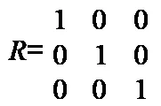
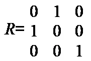
Moving a 1 within its column renames axes. Rows are the raw axes (x*, y*, z*) and columns the calibrated axes (x, y, z); this matrix swaps x and y:
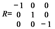
Changing the sign of a 1 reverses that axis; this matrix reverses x and z:
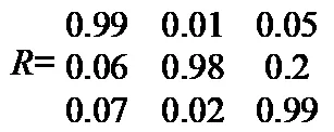
Values slightly away from 0 and 1 correct for axes that are not quite at right angles, as calculated by the accelerometer and gyroscope calibrations:
Sensitivity matrix
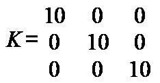
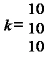
The sensitivity matrix K holds each axis’s sensitivity on its diagonal, with zeros elsewhere; it is the sensitivity vector k written as a matrix for convenience:
Offset vector
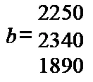
The offset vector b holds each axis’s reading at zero input:
How the parameters are found
For the gyroscope, the offset is the average output while the Shimmer is stationary. Each full turn about an axis is a rotation of known angle (2π), so integrating the gyroscope’s output, less its offset, over each of the three turns gives a 3×3 matrix of measured angles. Because each row of the alignment matrix is a unit vector, that matrix separates into the sensitivities and the alignment matrix.
For the accelerometer, the six static positions put gravity, a known quantity (Consensys takes it as 9.8 m/s²), along each axis in each direction. The sum of each pair of opposite readings gives the offsets, and their difference gives a matrix that separates, again using the unit-length rows of the alignment matrix, into the sensitivities and the alignment matrix.
For the magnetometer, readings taken in many orientations in an even field should all lie on a sphere whose radius is the field’s strength. For each axis, the midpoint of its highest and lowest readings gives the offset, and half their difference the sensitivity, so that the local field has a strength of 1. The alignment matrix is not measured (Section 6.4).
The accelerometer and gyroscope derivations are in the paper cited in Section 6.4.
For how to calibrate the kinematic sensors in Consensys, see Section 6.4.↩︎
Note that the LSM303DLHC accelerometer provides 12-bit resolution if HR mode is enabled and 10-bit resolution otherwise. The data is output in 16-bit format.↩︎
Note that the LSM303DLHC magnetometer provides 12-bit resolution. The data is output in 16-bit format.↩︎
Legal notices
Legal Notices and Disclaimer
Redistribution IS permitted provided that the following conditions are met:
Redistributions must retain the copyright notice, and the following disclaimer. Redistributions in electronic form must reproduce the above copyright notice, this list of conditions and the following disclaimer in the documentation and/or other materials provided with the document.
Neither the name of Shimmer Research Ltd. nor the names of its contributors may be used to endorse or promote products derived from this document without specific prior written permission.
THIS DOCUMENT IS PROVIDED BY THE COPYRIGHT HOLDERS AND CONTRIBUTORS “AS IS” AND ANY EXPRESS OR IMPLIED WARRANTIES, INCLUDING, BUT NOT LIMITED TO, THE IMPLIED WARRANTIES OF MERCHANTABILITY AND FITNESS FOR A PARTICULAR PURPOSE ARE DISCLAIMED. IN NO EVENT SHALL THE COPYRIGHT OWNER OR CONTRIBUTORS BE LIABLE FOR ANY DIRECT, INDIRECT, INCIDENTAL, SPECIAL, EXEMPLARY, OR CONSEQUENTIAL DAMAGES (INCLUDING, BUT NOT LIMITED TO, PROCUREMENT OF SUBSTITUTE GOODS OR SERVICES; LOSS OF USE, DATA, OR PROFITS; OR BUSINESS INTERRUPTION) HOWEVER CAUSED AND ON ANY THEORY OF LIABILITY, WHETHER IN CONTRACT, STRICT LIABILITY, OR TORT (INCLUDING NEGLIGENCE OR OTHERWISE) ARISING IN ANY WAY OUT OF THE USE OF THIS DOCUMENT, EVEN IF ADVISED OF THE POSSIBILITY OF SUCH DAMAGE.
